Table of Contents
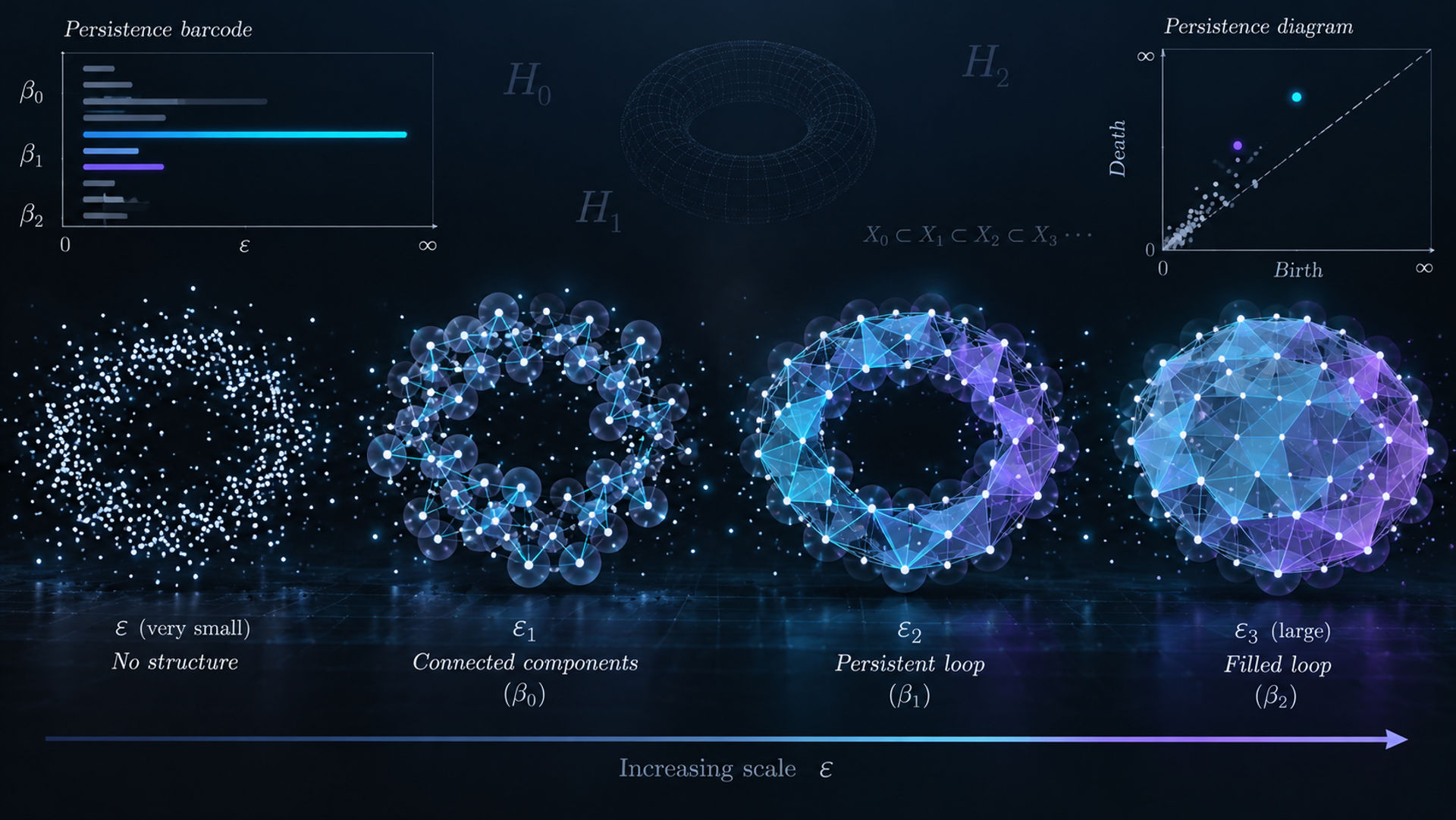
The computational engine behind topological data analysis, built up from geometric intuition

Take a scatter plot of points sampled noisily around a circle. Compute the mean: it lands near the center, a point that is not actually part of the data and tells you nothing about the ring-shaped structure surrounding it. Compute the variance in each direction: roughly equal, suggesting a formless blob. Run a linear correlation: close to zero, because a circle has no linear trend. Every standard descriptive statistic looks at this data and reports "nothing here" — while the shape of the data, a loop with a hole in the middle, is sitting in plain sight.
Persistent homology is the tool built specifically to see that hole. It is the central computational technique in topological data analysis (TDA), a field that treats a dataset not as a cloud of numbers to be averaged but as a geometric object whose connectivity, loops, and enclosed voids carry information. This article works through what persistent homology actually computes, how the algorithm proceeds step by step, and where it succeeds and fails as a data-analysis tool. It is the mechanical deep-dive beneath MathLumen's broader introduction to topological data analysis, which frames why shape-based methods matter; this piece is about how the pipeline actually works.
Topology is the branch of mathematics that studies properties preserved under continuous deformation — stretching, bending, compressing — but not under tearing or gluing. A coffee cup and a donut are topologically identical because one can be continuously deformed into the other (both have exactly one hole); a coffee cup and a plate are not, because you would have to tear the handle off or punch a hole through the plate to make them match.
This indifference to smooth distortion is exactly what makes topology useful for real data. Measured distances in a dataset are usually unreliable: sensor noise, measurement error, and arbitrary choices of coordinate system all stretch and jitter the raw numbers. A method that only cares about connectivity and enclosed structure, and is insensitive to the exact metric distortions layered on top, is far more robust to this kind of noise than a method that takes every coordinate literally.
A finite set of points sampled from an underlying shape is, by itself, topologically uninteresting — a discrete set of points has no loops or voids to speak of. To recover the shape the points were sampled from, persistent homology builds a simplicial complex: a combinatorial object made of vertices, edges, filled triangles, filled tetrahedra, and their higher-dimensional analogues (simplices), assembled according to a rule based on proximity.
The most common construction is the Vietoris–Rips complex. Fix a distance threshold . Connect two points with an edge if their distance is at most . Then, whenever all pairwise distances among a set of points are within of one another, fill in the corresponding -simplex — a triangle for three mutually close points, a tetrahedron for four, and so on. The Vietoris–Rips complex is popular in practice because it is cheap to build: it only requires pairwise distances, not any geometric information about balls in the ambient space.
A closely related construction is the Čech complex, built by placing a ball of radius around every point and forming a simplex whenever a collection of balls has nonempty common intersection. The Čech complex has a stronger theoretical guarantee — the Nerve Theorem says it is homotopy equivalent to the union of the balls themselves, so it faithfully reflects the shape those balls trace out — but computing common intersections of many balls is significantly more expensive than checking pairwise distances, which is why the Vietoris–Rips complex is the default choice for large datasets in practice, sometimes with the Čech complex used to sanity-check results on smaller ones.
Here is the difficulty: the choice of matters enormously, and there is no principled way to pick a single "correct" value in advance. Set too small and the complex is just a scatter of isolated points with no edges at all — every point is its own disconnected component. Set too large and every point ends up connected to every other point, collapsing any interesting loop or void into a single solid blob with no topological features left to detect.
The insight that makes persistent homology work is to stop trying to guess the right and instead sweep through all of them. As grows continuously from to some large value, the simplicial complex grows monotonically: edges appear, then triangles fill in, then tetrahedra, in a nested sequence called a filtration. Persistent homology examines this entire filtration at once rather than any single snapshot of it.
At each fixed value of , the simplicial complex has a well-defined shape, and algebraic topology gives a precise way to count its features using homology groups. In practice, what gets reported is a sequence of non-negative integers called Betti numbers, one for each dimension:
Higher Betti numbers ( and beyond) generalize the same idea to higher-dimensional holes, though they are rarely interpretable by eye and appear mainly in high-dimensional data analysis. Concretely: a single blob of merged points has and ; a ring has , ; a hollow sphere's surface has , , . Formally, is the rank of the -th homology group of the complex, computed via the boundary maps between chains of -simplices — but the geometric reading (pieces, loops, voids) is what a practitioner actually uses.
As increases through the filtration, individual topological features are born and die. A loop might not exist at , appear once enough edges have formed a ring at , and then die at once enough additional edges fill in the interior of the ring and collapse the hole. The persistence of that feature is the length of the interval between its birth scale and its death scale: .
The standard interpretive heuristic — and it is a heuristic, not a theorem — is that features with long persistence, surviving across a wide range of scales, represent genuine structure in the underlying shape the data was sampled from, while features with short persistence are artifacts of noise or of the specific finite sample. This is a reasonable default because real geometric structure tends to be visible across many nearby scales, while a spurious gap or accidental near-alignment of a few noisy points tends to appear and vanish quickly. It is not, however, an absolute rule: in some applications a swarm of short-lived features carries meaningful information about local texture or density variation, and dismissing every short bar as noise can throw away real signal. Persistence is a coordinate for ranking candidate features by robustness, not a hard cutoff for truth.
Persistent homology's output is typically displayed one of two equivalent ways.
A persistence diagram is a scatter plot where each topological feature is a single point, with its birth scale on the horizontal axis and its death scale on the vertical axis. Because death always occurs at or after birth, every point lies on or above the diagonal line . Points far from the diagonal correspond to long-lived, high-persistence features; points close to the diagonal correspond to short-lived features that are usually — again, not always — treated as noise.
A barcode conveys the same information differently: each feature is drawn as a horizontal line segment stretching from its birth value to its death value on a shared horizontal scale axis, with one bar per feature stacked vertically. Long bars are long-lived features; a barcode with one very long bar in the dimension and a cluster of short bars everywhere else is the classic signature of "one real loop plus sampling noise."
Both representations carry identical information; the choice between them is largely visual preference, though barcodes make it easier to compare many features' lifetimes at a glance, while diagrams make it easier to apply distance metrics (such as the bottleneck or Wasserstein distance between two diagrams) for statistical comparison.
Genuine strengths. Persistent homology is robust to the specific choice of distance metric and to moderate amounts of noise, because small perturbations to the data shift points in a persistence diagram only slightly — a fact made precise by stability theorems relating perturbation size to bottleneck distance between diagrams. It detects structure that is invariant under continuous deformation, so it does not care whether a loop in the data is a perfect circle or a lopsided oval, only that a loop is there. And because it operates across all scales simultaneously, it sidesteps the single-bandwidth problem that afflicts many clustering and density-estimation methods.
Genuine limitations. Computing persistent homology scales poorly: building the full simplicial complex and its filtration can require far more memory and computation than the size of the original dataset, particularly in high ambient dimension, where the number of possible simplices grows combinatorially. A dataset of points can, in principle, generate a Vietoris–Rips complex with exponentially many simplices in once high-dimensional faces are included, which is why practical implementations cap the maximum simplex dimension they track and rely on optimized boundary-matrix reduction algorithms rather than a naive computation of every homology group from scratch. This computational ceiling is the main reason persistent homology is typically applied to datasets of thousands, not millions, of points, or to data that has first been reduced in dimension or subsampled with landmark points chosen to preserve the overall shape. The result is also sensitive to how the data is embedded and which distance function is chosen — persistent homology reveals the shape of the representation you feed it, and a poor embedding will produce a topologically uninteresting or misleading answer even if the underlying phenomenon has real structure. And critically, a persistence diagram by itself does not constitute a statistical claim: seeing a long bar in a barcode does not establish, in a hypothesis-testing sense, that a dataset "has a loop" any more than seeing a cluster on a scatter plot establishes statistical significance. Rigorous use of TDA pairs the diagram with a statistical test — commonly one based on bottleneck or Wasserstein distance between the observed diagram and diagrams generated under a null model — before treating a feature as more than suggestive.
Persistent homology has moved beyond a purely theoretical curiosity into domains where geometric structure is genuinely hard to capture with standard statistics. In neuroscience, researchers have applied it to neural activity data to characterize the structure of correlations among firing neurons, looking for loop-like patterns that reflect the geometry of the underlying stimulus space rather than pairwise correlation alone. In structural biology, TDA methods have been used to study conformational flexibility in protein structures, where persistent loops in a configuration space can correspond to functionally relevant motions. In sensor network analysis, persistent homology (developed in this context largely through the work of Robert Ghrist and collaborators) has been used to verify coverage — determining whether a network of sensors with only local, coordinate-free connectivity information has fully covered a region, without needing to know each sensor's exact position. Financial time series analysis has also used persistence diagrams derived from sliding windows of market data as an early-warning signal ahead of periods of instability, on the premise that topological structure in the data changes character before a crash becomes visible in price alone. Each of these applications treats the persistence diagram as one input among several, combined with domain-specific statistical validation, rather than as a standalone proof of structure.
This article has focused on the mechanics: how a point cloud becomes a filtration, how a filtration becomes Betti numbers across scale, and how those numbers become a persistence diagram or barcode. For the broader context — why topological methods emerged as a response to the limitations of purely statistical data analysis, and how TDA relates to other approaches to finding structure in high-dimensional data — see MathLumen's introduction to topological data analysis. Readers coming from a machine learning background who want to see persistence diagrams used as features inside a learning pipeline (through vectorizations such as persistence landscapes or persistence images) should watch for a forthcoming piece on TDA and machine learning, which this article serves as the technical prerequisite for.

Applied mathematician and AI practitioner. Founder of MathLumen, exploring mathematics behind machine learning and scientific AI.
When Fourier meets computation
Spectral methods transform PDEs into algebraic systems using global basis functions. We survey how Fourier and...

Random walks on Wall Street — literally
Monte Carlo simulation is the backbone of derivatives pricing. We explore the mathematics of random sampling, variance...

Why your online banking depends on abstract algebra
Elliptic curve cryptography provides the strongest security per bit of any known public-key system. We explore the...